ERA Yield Stability
2025-04-02
ERA-Yield-Stability.RmdIn this vignette we will explore how to plot and calculate absolute and relative outcome stability.
Access the data
First we access the compiled ERA dataset included with the ERA package.
knitr::kable(head(ERAg::ERA.Compiled[,1:8], 5))| Index | Code | Author | Date | Journal | DOI | Elevation | Country |
|---|---|---|---|---|---|---|---|
| 1 | NN0001 | Bationo A | 1997 | NUTR CYCL AGROECOSYS | 10.1023/a:;1009784812549 | NA | Mali |
| 5 | NN0001 | Bationo A | 1997 | NUTR CYCL AGROECOSYS | 10.1023/a:;1009784812549 | NA | Mali |
| 9 | NN0001 | Bationo A | 1997 | NUTR CYCL AGROECOSYS | 10.1023/a:;1009784812549 | NA | Mali |
| 13 | NN0001 | Bationo A | 1997 | NUTR CYCL AGROECOSYS | 10.1023/a:;1009784812549 | NA | Mali |
| 17 | NN0001 | Bationo A | 1997 | NUTR CYCL AGROECOSYS | 10.1023/a:;1009784812549 | NA | Mali |
Our analyses of outcome stability are inspired and based on the publication A global meta-analysis of yield stability in organic and conservation agriculture by Knapp et al. 2018. As such we will be exploring the outcome subindicator crop yield in this vignette, which is a data rich vein in ERA.
Rename higher level concepts
Many functions in the ERA package have been designed work with standardized column names for the higher level concepts of practice, outcome and product (or experimental units) found in the ERA organizational hierarchy.
We can view the subordinates of these high level concepts by
accessing the internal datasets PracticeCodes,
OutcomesCodes and EUCodes.
| Code | Theme | Theme.Code | Practice | Practice.Code | Subpractice |
|---|---|---|---|---|---|
| a1 | Agroforestry | Agroforestry | FMNR | FMNR | Farmer Managed Natural Regeneration |
| a3 | Agroforestry | Agroforestry | Alleycropping | Al | Alleycropping (N fixing) |
| a4 | Agroforestry | Agroforestry | Alleycropping | Al | Alleycropping (Non N fixing) |
| a4.1 | Agroforestry | Agroforestry | Alleycropping | Al | Alleycropping (Mixed) |
| a14 | Agroforestry | Agroforestry | Alleycropping | Al | Alleycropping (Unspecified) |
Alternatively the organization of higher level concepts can also be
viewed in the ERAConcepts list.
ERAg::ERAConcepts
#> $Prac.Levels
#>         Choice Choice.Code      Prac           Base
#>         <char>      <char>    <char>         <char>
#> 1: Subpractice           S SubPrName SubPrName.Base
#> 2:    Practice           P    PrName    PrName.Base
#>
#> $Out.Levels
#>          Choice Choice.Code           Out
#>          <char>      <char>        <char>
#> 1: Subindicator          SI    Out.SubInd
#> 2:    Indicator           I       Out.Ind
#> 3:    Subpillar          SP Out.SubPillar
#> 4:       Pillar           P    Out.Pillar
#>
#> $Prod.Levels
#>     Choice Choice.Code            Prod
#>     <char>      <char>          <char>
#> 1: Product           P  Product.Simple
#> 2: Subtype           S Product.Subtype
#> 3:    Type           T    Product.Type
#>
#> $Agg.Levels
#>         Choice Choice.Code      Agg            Label
#>         <char>      <char>   <char>           <char>
#> 1: Observation           O    Index    No. Locations
#> 2:       Study           S     Code      No. Studies
#> 3:    Location           L Site.Key No. Observations
To apply standardized column names we need to select which
organizational levels of the three higher level concepts to use using
the StandColName function. The function help describes how
to do this ?StandColNames.
Crop yield is an outcome in the subindicator level of the
outcome hierarchy, so we set the OLevel parameter to
SI. In general you will be using the subindicator
level for stability analyses.
Regarding practices there are a large number of concepts at the
subpractice level, so let’s aggregate analysis up the
practice level; we set the PLevel parameter to
P.
The stability analysis does not explicitly consider products so it’s
not critical what organization level of prodct we choose; let’s set the
EULevel parameter to P.
StabData<-ERAg::StandColNames(Data=ERAg::ERA.Compiled,
              PLevel="P",
              OLevel="SI",
              EULevel="P"
              )
All we have done with the StandColNames function is to
rename columns, for example the Out.SubInd column has been
renamed Outcome.
To explore outcome x practice stability for specific products or
product groups we could subset the dataset on the products
columns, for example:
StabData<-StabData[Product.Subtype=="Cereals"]Prepare the data
Next we need to prepare the data for use with the
StabCalc2 function. To do this we use the
PrepareStabData function which labels multi-year
observations (MYO) and calculates means and variances for outcomes
within these MYOs. A multi-year observation is a pair of control and
experimental treatments, in the same place and study with multiple
observations of the same outcomes over time.
By default the PrepareStabData function subsets data to
the crop yields outcome (code=101), but the OutCodes
argument can be used to consider other outcomes. We can investigate
outcome codes in the OutcomeCodes dataset.
data.table(OutcomeCodes)[grep("Crop Yield",Subindicator),list(Subindicator,Code)]
#>    Subindicator  Code
#>          <char> <num>
#> 1:   Crop Yield   101
StabData<-ERAg::PrepareStabData(Data=StabData,OutCodes=101)The stability analysis needs MYOs of at least 3 seasons to generate
any statistics and the StabCalc function will filter any
MYOs that do not meet this minimum data requirement. If you want to
increase the thresholds for MYO length then you can filter on the
nryear field of the PrepareStabData output.
For example:
StabData<-StabData[nryears>=4]Plot the data
Now we use the ERAStabPlot function to plot the data,
this function creates a list of plots, one for each combination of
product x outcome.
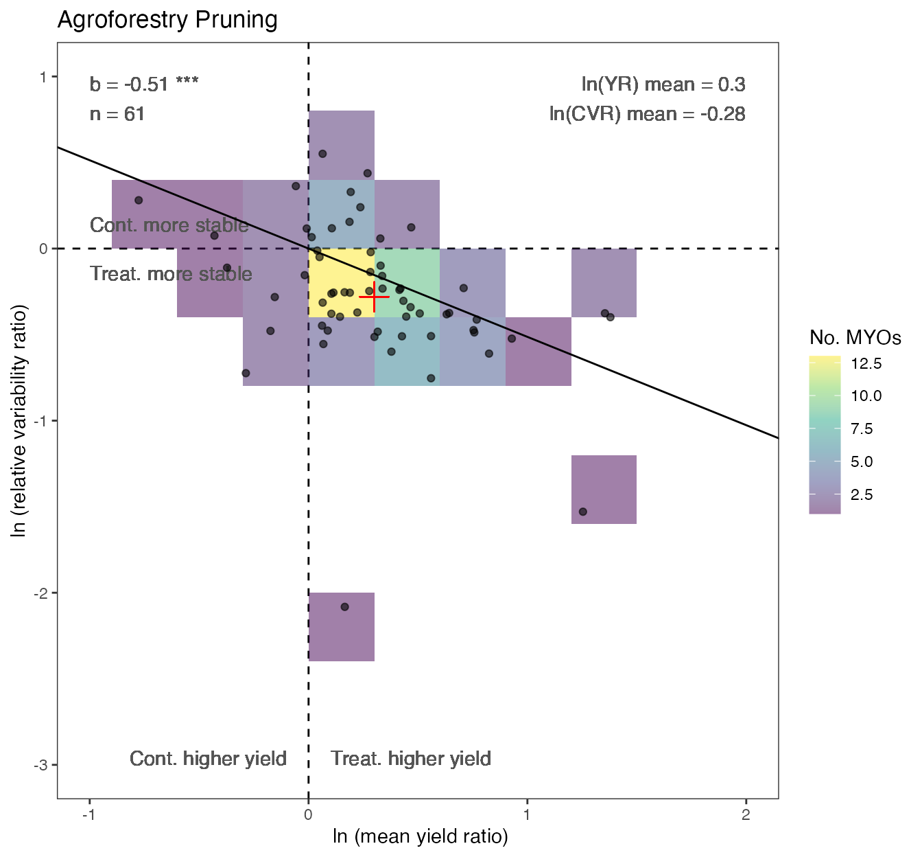
StabPlots<-ERAgON::ERAStabPlot(Data=StabData,Robust=F,Intercept=F)Each list element contains two elements, these are ggplots of 1)
absolute yield variability (lnVR) vs. yield
(lnRR) and 2) relative yield variability
(lnCVR) vs. yield (lnRR).
plot(StabPlots$`Crop Yield.Agroforestry Pruning`$lnVR)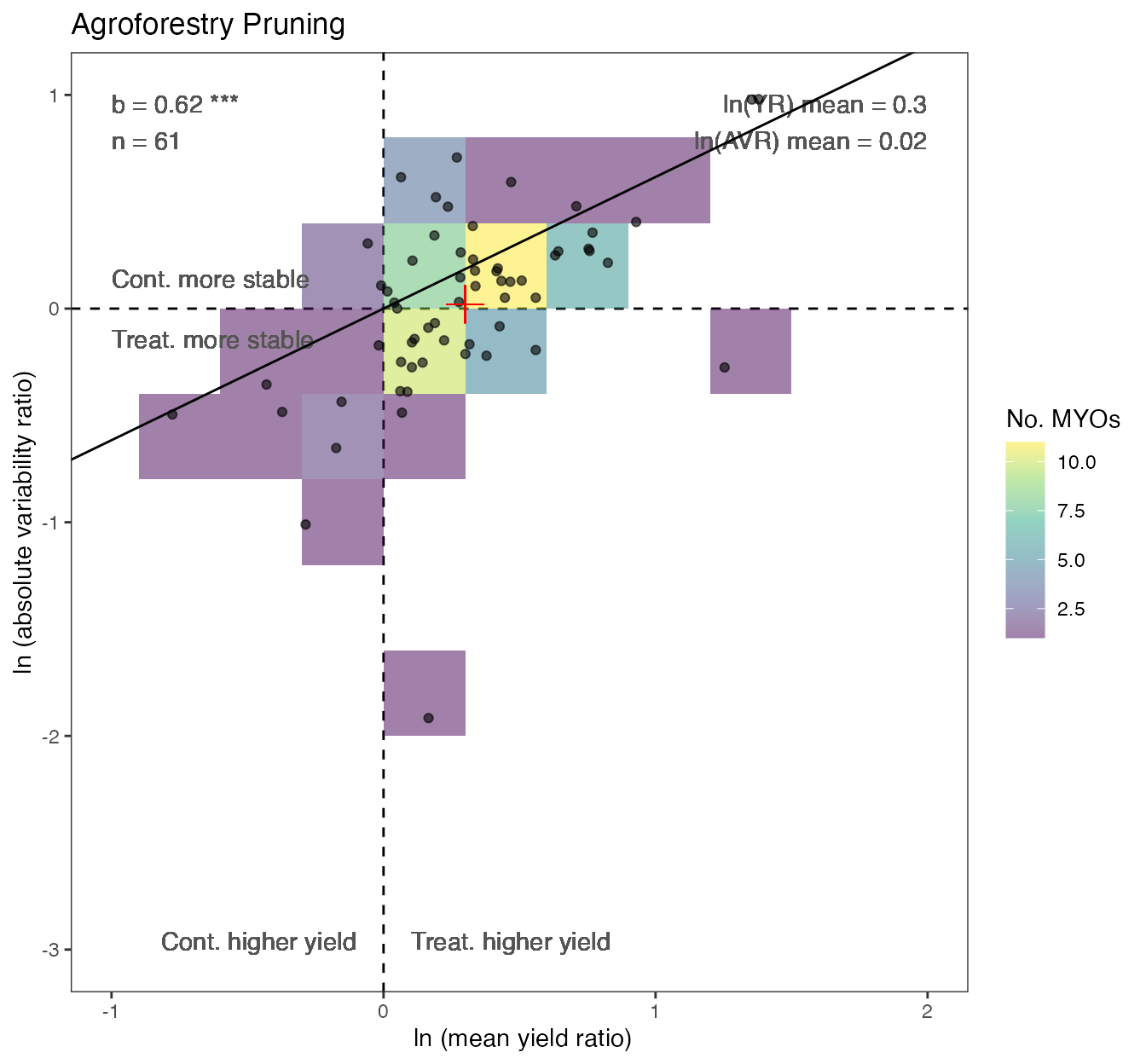
plot(StabPlots$`Crop Yield.Agroforestry Pruning`$lnCVR)